Usage
scATS can analyze both single-end and paired-end 5’-end scRNA-seq data, enabling direct quantification using Seurat objects, while incorporating RNA degradation (RD) modeling through expectation-maximization (EM).
The main functions of scATS are: TSSCDF, FindMarkersByTheta,FindMarkers, ThetaByGroup,psi, Sashimi
TSS inference and quantification
The input files include:
Seurat object (R object)
Alignment file (bam file)
Annotation file (gtf file)
# load packages
suppressMessages({
  library(scATS)
  library(Seurat)
  library(data.table)
})

# load input files
seu <- readRDS("demo/demo_seurat.Rds")
Genes <- rownames(seu)
gtfFile <- file.path("demo/demo.gtf")
bams <- "demo/demo.bam"
file.exists(bams)

# quantification using wrapper function
scats <- TSSCDF(object = seu, bam = bams, gtf = gtfFile, genes = Genes, verbose = TRUE, scDR = TRUE, UTROnly = TRUE)
scats
class: scATSDataSet
dim: 6 2000
metadata(2): version parameters
assays(4): counts psi theta alpha
rownames(6): OR4F5@1:69071:+ OR4F5@1:69090:+ ... SCNN1D@1:1287217:+ SCNN1D@1:1287223:+
rowData names(12): TSS gene_id ... alpha theta
colnames(2000): TGGACGCTCCTTCAAT-1 CGAGCACGTCAGAATA-1 ... ATCGAGTAGCGGCTTC-1 CTAGAGTAGTGCCATT-1
colData names(4): orig.ident nCount_RNA nFeature_RNA CellType
The quantification results are stored in scats@rowRanges and contain the following columns:
column name |
content |
|---|---|
seqnames |
The chromosomal name of the gene to which TSS belongs. |
ranges |
The genomic locus of TSS, where the growth rate is highest. |
strand |
The genomic strand of the gene to which TSS belongs. |
gene_id |
The Ensembl ID of the gene to which TSS belongs. |
gene_name |
The HGNC Symbol of the gene to which TSS belongs. |
TSS |
The ID of the TSS in the format of [seqnames:ranges:strand]. |
Region |
The growth area of the sorted 5’-starts of read 1, or it can also be interpreted as the |
PSI |
The percent spliced in (PSI) of TSS. |
Percent |
The ratio of TSS reads. |
Annotated |
The nearest annotated TSS locus that exists in the region, if it is NA, |
Greedy |
Greedy for the first TSS. If it is TRUE, it indicates that the first TSS is quantified |
beta |
The area under the cumulative distribution curve : close to 1, indicates no degradation, |
alpha |
The degradation index fitted using the EM algorithm: the larger the value, the more severe the degradation. |
theta |
The PSI value fitted using the EM algorithm. |
AllReads |
The total number of reads used for quantification. |
Note : All the following analyses are based on the scats object.
Finding differentially expressed ATSs
Finding markers of all group
Identifying ATS markers based on θ value.
DE <- scATS::FindMarkersByTheta(object = scats, groupBy = "CellType", group1 = NULL, group2 = NULL, cores = 20)
DE
     gene      TSS           group1 theta1   theta2   cell1  cell2 percent1 percent2     p
    <char>    <char>         <char> <num>    <num>    <int>  <int> <num>     <num>     <num>
1:  OR4F5 OR4F5@1:69063:+      A 0.3090495 0.2476250    14     9 1.3725490 0.9183673 0.2824086
2:  OR4F5 OR4F5@1:69063:+      B 0.2476250 0.3090495     9    14 0.9183673 1.3725490 0.2824086
3:  OR4F5 OR4F5@1:69071:+      A 0.2092985 0.3593406    12    17 1.1764706 1.7346939 0.1862959
4:  OR4F5 OR4F5@1:69071:+      B 0.3593406 0.2092985    17    12 1.7346939 1.1764706 0.1862959
5:  OR4F5 OR4F5@1:69080:+      A 0.1622722 0.1533179     9     9 0.8823529 0.9183673 0.9162350
6:  OR4F5 OR4F5@1:69080:+      B 0.1533179 0.1622722     9     9 0.9183673 0.8823529 0.9162350
The DE object contains following columns:
column name |
content |
|---|---|
gene |
The HGNC Symbol of the gene to which TSS belongs. |
TSS |
The ID of the TSS in the format of [gene_name:seqnames:ranges:strand]. |
group1 |
The levels of group. |
theta1/2 |
The theta value of the TSS in the group. |
cell1/2 |
The number of cell-type corresponding to group. |
percent1/2 |
The ratio of TSS reads. |
p |
The p-value from the Wilcoxon test for differences in psi values among groups. |
Identifying ATS markers based on ψ value.
DE <- scATS::FindMarkers(object = scats, groupBy = "CellType", group1 = NULL, group2 = NULL, cores = 20, majorOnly = F)
DE
    TSS                 G1     G2    n1    n2    N1    N2   Cells1  Cells2   PSI1   PSI2     PseudobulkPSI1
    <char>            <char> <char> <int> <int> <int> <int>  <int>  <int>   <num>   <num>          <num>
1: OR4F5@1:69071:+      A  Other    66    58   226   207   1020    980 0.2306640 0.2385772      0.2010582
2: OR4F5@1:69071:+      B  Other    58    66   207   226    980   1020 0.2385772 0.2306640      0.3260394
    PseudobulkPSI2 wald.test  wilcox.test  prop.test
          <num>     <num>       <num>      <num>
1:      0.3260394 0.9230017   0.9005852 1.279065e-09
2:      0.2010582 0.9230017   0.9005852 1.279065e-09
The DE object contains following columns:
column name |
content |
|---|---|
TSS |
The ID of the TSS in the format of [gene_name:seqnames:ranges:strand]. |
G1/2 |
The levels of group. |
n1/2 |
The expression number of the TSS in the G1/2. |
N1/2 |
The expression number of the host gene in the G1/2. |
Cells1/2 |
The number of cell-type corresponding to G1/2. |
PSI1/2 |
The average sum of all individual cell PSIs. |
PseudobulkPSI1/2 |
The PSI value calculated by combining all reads and treating them as a pseudobulk sample. |
wald.test |
The p-value from the Wald test for differences in psi values among groups. |
wilcox.test |
The p-value from the Wilcoxon test for differences in psi values among groups. |
prop.test |
The p-value from the Proportion test for differences in psi values among groups. |
Finding markers of given group
### based on θ value
DE <- scATS::FindMarkersByTheta(object = scats, groupBy = "CellType",group1 = "A", group2 = "B", cores = 20)
### based on  ψ value
DE <- scATS::FindMarkers(object = scats, groupBy = "CellType", group1 = "A", group2 = "B", cores = 20, majorOnly = F,gene = "OR4F5")
In addition, you can specify the host genes used in the calculation by setting the gene parameter.
Calculating PSI
Calculating PSI based on θ value.
theta <- scATS::ThetaByGroup(object = scats, gene = "OR4F5",groupBy = "CellType")
theta
      Group    TSS     alpha    theta
      <char>  <char>   <num>    <num>
1:      A 1:69090:+ 0.3766315 0.4308618
2:      A 1:69071:+ 0.9681916 0.5691382
3:      B 1:69090:+ 0.2349261 0.1561318
4:      B 1:69071:+ 0.6822974 0.8438682
Calculating PSI based on ψ value.
psi <- scATS::psi(object = scats, groupBy = "CellType", TSS=c("OR4F5@1:69071:+", "OR4F5@1:69090:+"))
psi
    TSS             groupBy Cells   N  n      mean      sd        se         ci       median Q1 Q3 mad iqr
1 OR4F5@1:69071:+       A  1020   105 66  0.5813757 0.4859188 0.04742081 0.09403726      1  0  1   0   1
2 OR4F5@1:69071:+       B   980   96  58  0.5856689 0.4889869 0.04990702 0.09907795      1  0  1   0   1
3 OR4F5@1:69090:+       A  1020   105 46  0.4186243 0.4859188 0.04742081 0.09403726      0  0  1   0   1
4 OR4F5@1:69090:+       B   980   96  42  0.4143311 0.4889869 0.04990702 0.09907795      0  0  1   0   1
   PseudobulkPSI
1     0.4935065
2     0.6436285
3     0.5064935
4     0.3563715
The theta or psi object contains following columns:
column name |
content |
|---|---|
Group/groupBy |
The level of group. |
TSS |
The ID of the TSS in the format of [gene_name:seqnames:ranges:strand]. |
alpha |
The degradation index fitted using the EM algorithm. |
Cells |
The number of cell-type corresponding to a given groups (The same applies to the following.). |
N |
The expression of the host gene. |
n |
The expression of the TSS. |
mean |
The mean of PSI. |
sd |
The standard deviation (std) of PSI. |
se |
The standard error (SE) of PSI. |
ci |
The confidence interval (CI) of PSI. |
median |
The median of PSI. |
Q1 |
The first quartile (Q1) of PSI. |
Q3 |
The third quartile (Q3) of PSI. |
mad |
The median absolute deviation (MAD) of PSI. |
iqr |
The interquartile range (IQR) of PSI. |
theta/PseudobulkPSI |
The PSI value calculated by combining all reads and treating them as a pseudobulk sample. |
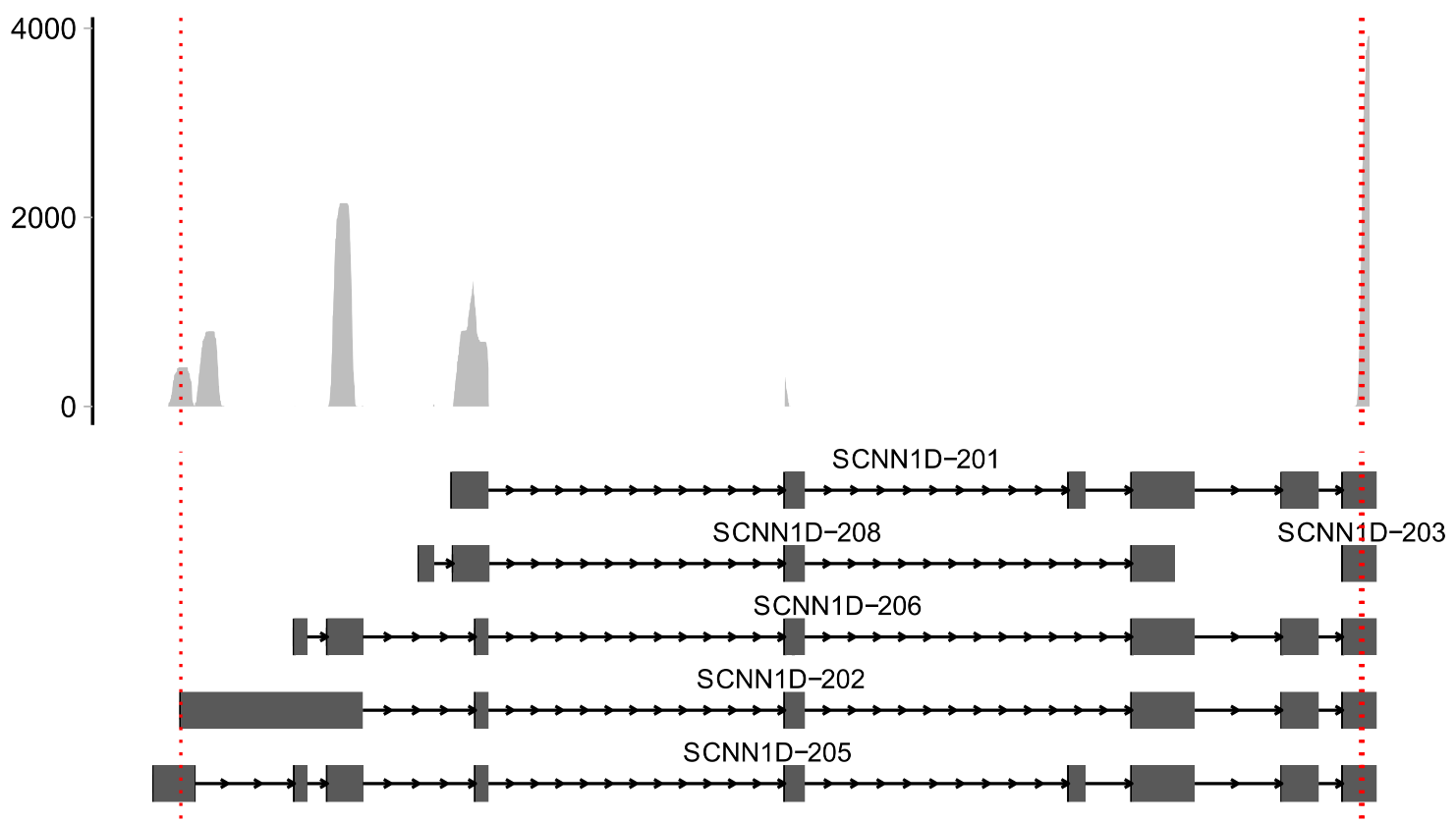
Sashimi plots
# Take SCNN1D gene as an example
gene_symbol <- "SCNN1D"
tss <- GenomicRanges::start(scats@rowRanges[scats@rowRanges$gene_name==gene_symbol])
scATS::Sashimi(object = scats,
               bam = bams,
               xlimit = c(1280352, 1287325),
               gtf = gtfFile,
               gene = gene_symbol,
               TSS = tss, # TSS位点
               free_y = T,#是否scale
               base_size = 12, #read部分字体大小
               rel_height=0.9, #注释/read ,小于1 read部分比例更大
               fill.color = "grey",
               line.color = "red",
               line.type = 3) -> p
p
sessionInfo()
    R version 4.5.2 (2025-10-31)
    Platform: x86_64-pc-linux-gnu
    Running under: Ubuntu 22.04.5 LTS

    Matrix products: default
    BLAS:   /usr/lib/x86_64-linux-gnu/blas/libblas.so.3.10.0
    LAPACK: /usr/lib/x86_64-linux-gnu/lapack/liblapack.so.3.10.0  LAPACK version 3.10.0

    locale:
    [1] LC_CTYPE=en_US.UTF-8       LC_NUMERIC=C
    [3] LC_TIME=zh_CN.UTF-8        LC_COLLATE=en_US.UTF-8
    [5] LC_MONETARY=zh_CN.UTF-8    LC_MESSAGES=en_US.UTF-8
    [7] LC_PAPER=zh_CN.UTF-8       LC_NAME=C
    [9] LC_ADDRESS=C               LC_TELEPHONE=C
    [11] LC_MEASUREMENT=zh_CN.UTF-8 LC_IDENTIFICATION=C

    time zone: Asia/Shanghai
    tzcode source: system (glibc)

    attached base packages:
    [1] stats     graphics  grDevices utils     datasets  methods   base

    other attached packages:
    [1] scATS_0.5.6

    loaded via a namespace (and not attached):
    [1] RcppAnnoy_0.0.22            splines_4.5.2
    [3] later_1.4.4                 BiocIO_1.20.0
    [5] filelock_1.0.3              bitops_1.0-9
    [7] tibble_3.3.0                R.oo_1.27.1
    [9] polyclip_1.10-7             graph_1.88.1
    [11] rpart_4.1.24                XML_3.99-0.20
    [13] fastDummies_1.7.5           httr2_1.2.2
    [15] lifecycle_1.0.4             OrganismDbi_1.52.0
    [17] ensembldb_2.34.0            globals_0.18.0
    [19] lattice_0.22-5              MASS_7.3-65
    [21] backports_1.5.0             magrittr_2.0.4
    [23] rmarkdown_2.30              Hmisc_5.2-4
    [25] plotly_4.11.0               yaml_2.3.12
    [27] httpuv_1.6.16               otel_0.2.0
    [29] Seurat_5.3.1                sctransform_0.4.2
    [31] spam_2.11-1                 sp_2.2-0
    [33] spatstat.sparse_3.1-0       reticulate_1.44.1
    [35] ggbio_1.58.0                cowplot_1.2.0
    [37] pbapply_1.7-4               DBI_1.2.3
    [39] RColorBrewer_1.1-3          abind_1.4-8
    [41] Rtsne_0.17                  GenomicRanges_1.62.1
    [43] mixtools_2.0.0.1            purrr_1.2.0
    [45] R.utils_2.13.0              AnnotationFilter_1.34.0
    [47] biovizBase_1.58.0           BiocGenerics_0.56.0
    [49] RCurl_1.98-1.17             nnet_7.3-20
    [51] rappdirs_0.3.3              VariantAnnotation_1.56.0
    [53] IRanges_2.44.0              S4Vectors_0.48.0
    [55] ggrepel_0.9.6               irlba_2.3.5.1
    [57] listenv_0.10.0              spatstat.utils_3.2-0
    [59] goftest_1.2-3               RSpectra_0.16-2
    [61] spatstat.random_3.4-3       fitdistrplus_1.2-4
    [63] parallelly_1.46.0           codetools_0.2-19
    [65] DelayedArray_0.36.0         tidyselect_1.2.1
    [67] UCSC.utils_1.6.1            farver_2.1.2
    [69] BiocFileCache_3.0.0         matrixStats_1.5.0
    [71] stats4_4.5.2                base64enc_0.1-3
    [73] spatstat.explore_3.6-0      Seqinfo_1.0.0
    [75] GenomicAlignments_1.46.0    jsonlite_2.0.0
    [77] progressr_0.18.0            Formula_1.2-5
    [79] ggridges_0.5.7              survival_3.8-3
    [81] progress_1.2.3              segmented_2.1-4
    [83] tools_4.5.2                 ica_1.0-3
    [85] Rcpp_1.1.0                  glue_1.8.0
    [87] gridExtra_2.3               SparseArray_1.10.8
    [89] xfun_0.55                   MatrixGenerics_1.22.0
    [91] GenomeInfoDb_1.46.2         dplyr_1.1.4
    [93] BiocManager_1.30.27         fastmap_1.2.0
    [95] digest_0.6.39               R6_2.6.1
    [97] mime_0.13                   colorspace_2.1-2
    [99] scattermore_1.2             tensor_1.5.1
    [101] biomaRt_2.66.0              dichromat_2.0-0.1
    [103] spatstat.data_3.1-9         RSQLite_2.4.5
    [105] cigarillo_1.0.0             R.methodsS3_1.8.2
    [107] tidyr_1.3.2                 generics_0.1.4
    [109] data.table_1.17.8           rtracklayer_1.70.0
    [111] prettyunits_1.2.0           httr_1.4.7
    [113] htmlwidgets_1.6.4           S4Arrays_1.10.1
    [115] uwot_0.2.4                  pkgconfig_2.0.3
    [117] gtable_0.3.6                blob_1.2.4
    [119] lmtest_0.9-40               S7_0.2.1
    [121] XVector_0.50.0              htmltools_0.5.9
    [123] dotCall64_1.2               RBGL_1.86.0
    [125] ProtGenerics_1.42.0         SeuratObject_5.3.0
    [127] scales_1.4.0                Biobase_2.70.0
    [129] png_0.1-8                   spatstat.univar_3.1-5
    [131] rstudioapi_0.17.1           knitr_1.51
    [133] reshape2_1.4.5              rjson_0.2.23
    [135] checkmate_2.3.3             nlme_3.1-168
    [137] curl_7.0.0                  cachem_1.1.0
    [139] zoo_1.8-15                  stringr_1.6.0
    [141] KernSmooth_2.23-26          parallel_4.5.2
    [143] miniUI_0.1.2                foreign_0.8-90
    [145] AnnotationDbi_1.72.0        restfulr_0.0.16
    [147] pillar_1.11.1               grid_4.5.2
    [149] vctrs_0.6.5                 RANN_2.6.2
    [151] VGAM_1.1-14                 promises_1.5.0
    [153] dbplyr_2.5.1                xtable_1.8-4
    [155] cluster_2.1.8.1             htmlTable_2.4.3
    [157] evaluate_1.0.5              GenomicFeatures_1.62.0
    [159] cli_3.6.5                   compiler_4.5.2
    [161] Rsamtools_2.26.0            rlang_1.1.6
    [163] crayon_1.5.3                future.apply_1.20.1
    [165] mclust_6.1.2                plyr_1.8.9
    [167] stringi_1.8.7               viridisLite_0.4.2
    [169] deldir_2.0-4                BiocParallel_1.44.0
    [171] txdbmaker_1.6.0             Biostrings_2.78.0
    [173] lazyeval_0.2.2              spatstat.geom_3.6-1
    [175] Matrix_1.7-4                BSgenome_1.78.0
    [177] RcppHNSW_0.6.0              hms_1.1.4
    [179] patchwork_1.3.2             bit64_4.6.0-1
    [181] future_1.68.0               ggplot2_4.0.1
    [183] KEGGREST_1.50.0             shiny_1.12.1
    [185] SummarizedExperiment_1.40.0 kernlab_0.9-33
    [187] ROCR_1.0-11                 igraph_2.2.1
    [189] memoise_2.0.1               bit_4.6.0